Taming Big Data: An Introduction to Apache Spark
By the time I reached the Big Data course in my master’s program, I’d built a solid foundation across multiple programming paradigms. Each one gave me a different lens for thinking about computation.
But none of them prepared me for the scale problem. What happens when your data doesn’t fit in one machine’s memory? When a single CPU can’t process your dataset before the next one arrives? When you need to coordinate hundreds of machines to answer a single query?
That’s the territory Apache Spark occupies. And for my Big Data course final project, I didn’t just study it — I built a complete teaching resource: a presentation with slides, interactive Jupyter notebooks covering the full Spark ecosystem, and a Docker-based cluster so anyone could run the examples on their own machine. The goal was to make the abstract concrete — to take a framework designed for clusters of hundreds of machines and make it approachable on a laptop.
The talk
The presentation covered Apache Spark from the ground up. I wanted classmates to walk away not just understanding what Spark does, but being able to write and run Spark programs themselves. The presentation slides provided the theoretical framework, but the real learning happened in the notebooks.
I structured the material as a progressive journey through Jupyter notebooks, each one building on the previous. The companion repository contains everything: the notebooks, the data files, and a Docker setup to spin up a local Spark cluster. The idea was that anyone could clone the repo and start experimenting immediately.
The reference book for the course was “Learning Spark” by Karau, Konwinski, Wendell, and Zaharia (O’Reilly, 2015) — still one of the best introductions to the framework.
What is Apache Spark?
Apache Spark started in 2009 at UC Berkeley’s AMPLab as a research project. It was open-sourced in 2010, transferred to the Apache Software Foundation in 2013, and became a Top-Level Project in February 2014. Version 1.0 shipped in May 2014. By the time I was studying it, Spark had already become the de facto standard for large-scale data processing.
The core promise is simple: take MapReduce’s model for distributed computation and make it faster. Spark achieves 10-20x speedups over Hadoop MapReduce for complex applications, primarily by keeping data in memory between operations instead of writing to disk after every step.
The architecture follows a master-worker pattern. A driver program creates a SparkContext — the connection to the cluster. The SparkContext communicates with a cluster manager (YARN, Mesos, or Spark’s standalone manager), which allocates resources across executor processes on worker nodes. Each executor runs tasks and stores data in memory.
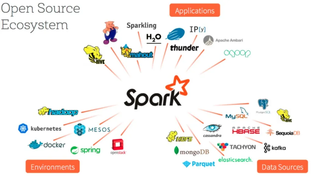
What makes Spark particularly powerful is its unified stack. On top of the core engine sit four libraries: Spark SQL for structured data, Spark Streaming for real-time processing, MLlib for machine learning, and GraphX for graph computation. One engine, four use cases, and they all share the same underlying abstraction.
RDDs — the foundation
Everything in Spark starts with the Resilient Distributed Dataset (RDD). An RDD is an immutable, distributed collection of elements that can be operated on in parallel. You don’t write loops to process data — you declare transformations, and Spark figures out how to distribute the work across the cluster.
Two things make RDDs special. First, they’re lazily evaluated: transformations don’t execute immediately. Instead, Spark builds up a directed acyclic graph (DAG) of operations and only executes when you call an action that needs a result. Second, they’re resilient: if a partition is lost due to a node failure, Spark can reconstruct it by replaying the transformations from the original data.
I used Don Quixote as the dataset for the early notebooks — a fun choice for a Spanish-speaking audience. Here’s a taste of what working with RDDs looks like:
# Create an RDD from a text file
rdd = sc.textFile("data/quijote.txt")

# Count words using transformations and actions
words = rdd.flatMap(lambda line: line.split(" "))
word_counts = words.map(lambda word: (word, 1)).reduceByKey(lambda a, b: a + b)
top_words = word_counts.takeOrdered(5, key=lambda x: -x[1])
That’s the MapReduce pattern distilled: flatMap splits lines into words, map creates key-value pairs, and reduceByKey aggregates by key — all distributed across the cluster automatically.
The notebooks went deep on transformations — map, filter, flatMap, union, intersection, subtract, cartesian — and actions — reduce, fold, aggregate, collect, count, take, top. Then came key-value pair RDDs with their own specialized operations: reduceByKey, groupByKey, combineByKey for computing averages, and all four join types — inner, left outer, right outer, and full outer.
Beyond the basics
Once the fundamentals were solid, the notebooks moved into more advanced territory.
Numeric RDDs showed how Spark has built-in statistical functions. I generated random values from a normal distribution and computed statistics — mean, standard deviation, variance — in a single call. Then I used the 3-sigma rule to detect outliers and visualized the distribution with matplotlib histograms.
The more interesting example was analyzing US patent data from 1963 to 1999. Using reduceByKey to count patents per year revealed a clear upward trend visualized as a bar chart.
# US patent analysis
patents = sc.textFile("data/apat63_99.txt")
us_patents = patents.filter(lambda line: '"US"' in line)
by_year = us_patents.map(lambda line: (line.split(",")[1], 1))
counts = by_year.reduceByKey(lambda a, b: a + b)
Persistence and partitioning addressed a critical performance concern: by default, Spark recomputes the entire lineage of transformations every time you call an action. For iterative algorithms — machine learning, graph processing — that’s prohibitively expensive. The solution is cache() or persist() with six storage levels ranging from MEMORY_ONLY to DISK_ONLY to OFF_HEAP, each trading off speed against memory usage and fault tolerance.
File I/O demonstrated Spark’s flexibility with data sources. The highlight was reading compressed Project Gutenberg books using wholeTextFiles, which returns each file as a single key-value pair (filename → contents), and then counting words per book — with varying word counts depending on the book.
Setting up a real cluster
Theory is one thing. Running Spark on an actual cluster is another.
I built a Docker-based cluster using the Big Data Europe community images, which made it possible for anyone to spin up a multi-node Spark environment without manual installation. The setup was straightforward with docker-compose:
version: "2"
services:
  spark-master:
    image: bde2020/spark-master:2.3.1-hadoop2.7
    ports:
      - "8090:8080"
      - "7077:7077"
  spark-worker-1:
    image: bde2020/spark-worker:2.3.1-hadoop2.7
    environment:
      - SPARK_MASTER=spark://spark-master:7077
  spark-worker-2:
    image: bde2020/spark-worker:2.3.1-hadoop2.7
    environment:
      - SPARK_MASTER=spark://spark-master:7077
  spark-worker-3:
    image: bde2020/spark-worker:2.3.1-hadoop2.7
    environment:
      - SPARK_MASTER=spark://spark-master:7077
One master node coordinating three workers, all connected through Spark’s native protocol on port 7077. The master’s web UI on port 8090 let you monitor jobs, stages, and executors in real time.
For deploying applications, spark-submit is the standard tool:
spark-submit --master spark://spark-master:7077 \
  --executor-memory 512m \
  --num-executors 3 \
  myscript.py
The notebook also covered YARN integration — both client mode (driver runs locally) and cluster mode (driver runs on the cluster) — and three ways to configure Spark: programmatically through SparkConf objects, via command-line flags, or through external properties files.
The ecosystem libraries
The final notebooks covered the libraries that make Spark more than just a MapReduce replacement.
Spark SQL
Spark SQL introduced DataFrames — distributed collections of named columns, conceptually similar to database tables or Pandas DataFrames. The key insight is that DataFrames carry schema information, which enables the Catalyst query optimizer and the Tungsten execution engine to produce dramatically faster execution plans than plain RDD operations.
from pyspark.sql import SQLContext

sqlContext = SQLContext(sc)
df = sqlContext.read.json("data/gente.json")
df.show()
# +----+-------+
# |edad| nombre|
# +----+-------+
# |  17|  Celia|
# |  53|   Juan|
# |  39|Manuela|
# |  17|    Ana|
# +----+-------+
Loading JSON, running SQL queries, and joining datasets — all with the optimizer working behind the scenes. DataFrames were positioned as the eventual replacement for raw RDDs, and history proved that right.
GraphX
GraphX handles graph-parallel computation. The main abstraction is a directed multigraph with properties on vertices and edges. I demonstrated it with a Simpsons family graph — Homer, Marge, Bart, and Milhouse connected by relationships like “father,” “mother,” “married to,” and “friend.”
One important limitation at the time: GraphX was only available in Scala, not PySpark. So this was the one notebook where we switched languages — a good excuse to show Scala’s syntax too.
Spark ML
Spark’s machine learning library comes in two flavors: spark.mllib (the original RDD-based API) and spark.ml (the newer DataFrame-based API). The KMeans clustering example made the concept tangible:
from pyspark.mllib.clustering import KMeans
from pyspark.mllib.linalg import SparseVector

data = sc.parallelize([
    SparseVector(3, {1: 1.2}),
    SparseVector(3, {1: 1.1}),
    SparseVector(3, {0: 0.9, 2: 1.0}),
    SparseVector(3, {0: 1.0, 2: 1.1})
])

model = KMeans.train(data, k=2, initializationMode="k-means||")
print(model.clusterCenters)
# [array([0.0, 1.15, 0.0]), array([0.95, 0.0, 1.05])]
The sparse vectors cleanly separated into two clusters. The model could then predict new points and be saved to disk for later use — the full ML pipeline from training to deployment.
Spark Streaming
The final notebook tackled real-time data processing with DStreams (discretized streams). Spark Streaming uses a micro-batch architecture: incoming data is grouped into batches at regular intervals, each batch becomes an RDD, and the full power of Spark’s engine processes them.
I built two versions of a network word counter reading from a TCP socket:
- Stateless: Each batch counted words independently using
reduceByKey— no memory between batches. - Stateful: Using
updateStateByKeywith checkpointing, word counts accumulated across batches, building a running total over time.
The difference between those two approaches captures something fundamental about stream processing: do you need to remember what happened before, or is each window self-contained?
What I learned
Preparing this talk taught me as much as any course lecture. When you have to explain something to others — and make it work live in notebooks — you can’t hide behind vague understanding. Every concept had to be concrete enough to demonstrate.
A few things stood out:
The abstraction is the achievement. Spark’s genius isn’t in any single algorithm — it’s in hiding the complexity of distributed systems behind a familiar programming interface. You write rdd.map(f).filter(g).reduce(h) and Spark handles partitioning, shuffling, fault tolerance, and scheduling across the cluster. The gap between writing a local program and a distributed one shrinks dramatically.
Lazy evaluation changes how you think. When transformations don’t execute immediately, you start thinking about computation as a graph of dependencies rather than a sequence of steps. The DAG optimizer can reorder, combine, and eliminate operations in ways you’d never do manually. You describe what you want; the engine decides how to get it.
The unified stack matters. Before Spark, doing SQL queries, machine learning, graph processing, and stream processing meant running four different systems. Spark puts them all on the same engine, with the same data abstractions. That’s not just convenient — it eliminates the data movement and format conversion that dominated pre-Spark big data architectures.
Hands-on beats slides. The notebooks were the most valuable part of the project. Slides explain concepts; notebooks let you experiment. Changing a parameter, adding a transformation, watching how the output changes — that’s where understanding forms. Every future talk I gave carried this lesson.
Looking back
This project came at a good point in my learning journey. I’d built enough foundation in programming paradigms to appreciate what Spark was doing differently. The functional concepts — map, filter, reduce — were literally the building blocks of RDD operations. The distributed systems concepts were new, but the programming patterns were familiar.
Apache Spark showed me that the ideas from single-machine programming don’t disappear at scale — they transform. Map is still map. Reduce is still reduce. The difference is that they’re running across a cluster, and there’s an engine between your code and the hardware that handles all the complexity you’d rather not think about.
The framework will keep evolving, but the fundamental concepts remain the same. RDDs, lazy evaluation, the DAG scheduler, the unified stack. Understanding those foundations will make every new version easier to grasp.
Let’s keep building.
Resources
- Apache Spark Introduction — Jupyter notebooks, Docker cluster, and data files (GitHub)
- Presentation slides — Introduction to Apache Spark
- “Learning Spark” by Karau, Konwinski, Wendell & Zaharia (O’Reilly, 2015)